Showing posts with label model. Show all posts

Oct 23, 2022

Why VaR fails and actuaries can do better

Perhaps the most important challenge of an actuary is to develop and train the capability to explain complex matters in a simple way. One of the best examples of practicing this 'complexity reduction ability' has been given by David Einhorn, president of Greenlight Capital. In a nutshell David explains with a simple example why VaR models fail. Take a look at the next excerpt of David's interesting article in Point-Counterpoint.

Why Var fails
A risk manager’s job is to worry about whether the bank is putting itself at risk in unusual times - or, in statistical terms, in the tails of the distribution. Yet, VaR ignores what happens in the tails. It specifically cuts them off. A 99% VaR calculation does not evaluate what happens in the last1%. This, in my view, makes VaR relatively useless as a risk management tool and potentially catastrophic when its use creates a false sense of security among senior managers and watchdogs.
VaR is like an airbag that works all the time, except when you have a car accident
By ignoring the tails, VaR creates an incentive to take excessive but remote risks.
Example
Consider an investment in a coin flip. If you bet $100 on tails at even money, your VaR to a 99% threshold is $100, as you will lose that amount 50% of the time, which obviously is within the threshold. In this case, the VaR will equal the maximum loss.

Compare that to a bet where you offer 127 to 1 odds on $100 that heads won’t come up seven times in a row. You will win more than 99.2% of the time, which exceeds the 99% threshold. As a result, your 99% VaR is zero, even though you are exposed to a possible $12,700 loss.

In other words, an investment bank wouldn’t have to put up any capital to make this bet. The math whizzers will say it is more complicated than that, but this is the idea. Now we understand why investment banks held enormous portfolios of “super-senior triple A-rated” whatever. These securities had very small returns. However, the risk models said they had trivial VaR, because the possibility of credit loss was calculated to be beyond the VaR threshold. This meant that holding them required only a trivial amount of capital, and a small return over a trivial capital can generate an almost infinite revenue-to-equity ratio. VaR-driven risk management encouraged accepting a lot of bets that amounted to accepting the risk that heads wouldn’t come up seven times in a row. In the current crisis, it has turned out that the unlucky outcome was far more likely than the backtested models predicted. What is worse, the various supposedly remote risks that required trivial capital are highly correlated; you don’t just lose on one bad bet in this environment, you lose on many of them for the same reason. This is why in recent periods the investment banks had quarterly write-downs that were many times the firm-wide modelled VaR.

The Real Risk Issues
What. besides the 'art of simple communication', can we - actuaries - learn from David Einhorn? What David essentially tries to tell us, is that we should focus on the real Risk Management issues that are in the x% tail and not on the other (100-x)%. Of course, we're inclined to agree with David. But are we actuaries truly focusing on the 'right' risks in the tail? I'm afraid the answer to this question is most often: No! Let's look at a simple example that illustrates the way we are (biased) focusing on the wrong side of the VaR curve.

Example Longevity
For years (decades) now, longevity risk has been structurally underestimated. Yes, undoubtedly we have learned some of our lessons. Today's longevity calculations are not (anymore) just based on simple straight-on mortality observations of the past. Nevertheless, in our search to grasp, analyze and explain the continuous life span increase, we've got caught in an interesting but dangerous habit of examining more and more interesting details that might explain the variance of future developments in mor(t)ality rates. As 'smart' longevity actuaries and experts, we consider a lot of sophisticated additional elements in our projections or calculations. Just a small inventory of actuarial longevity refinement:
  • Difference in mortality rates: Gender, Marital or Social status, Income or Health related mortality rates
  • Size: Standard deviation, Group-, Portfolio-size
  • Selection effects, Enhanced annuities
  • Extrapolation: Generation tables, longitudinal effects, Autocorrelation, 'Heat Maps'
X-Tails In our increasing enthusiasm to capture the longevity monster, we got engrossed in our work. As experienced actuaries we know the devil is always in the De-Tails, however the question is: In which details? We all know perfectly well that probably the most essential triggers for longevity risk in the future, can not be found in our data. These triggers depend on the effect of new developments like :

It's clear that investigating and modeling the soft risk indicators of extreme longevity is no longer a luxury, as also an exploding increase in lifespan of 10-20% in the coming decades seems not unlikely. By stretching our actuarial research to the medical arena, we would be able to develop new (more) future- and shock-proof longevity models and stress tests. Regrettably, we don't like to skate on thin ice..... Ostrich Management If we - actuaries - would take longevity and our profession as 'Risk Manager' more seriously, we would warn the world about the global estimated (financial) impact of these medical developments on Pension- and Health topics. We would advise on which measures to take, in order to absorb and manage this future risk. Instead of taking appropriate actions, we hide in the dark, maintaining our belief in Fairy-Tails. As unworldly savants, we joyfully keep our eyes on the research of relative small variances in longevity, while neglecting the serious mega risks ahead of us. This way of Ostrich Management is a worrying threat to the actuarial profession. As we are aware of these kinds of (medical) future risks, not including or disclaiming them in our models and advice, could even have a major liability impact. In order to be able to prevent serious global loss, society expects actuaries to estimate and advise on risk, instead of explaining afterward what, why and how things went wrong, what we 'have learned' and what we 'could or should' have done. 
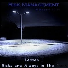
This way of denying reality reminds me of an amusing Jewish story of the Lost Key...

The lost Key
One early morning, just before dawn, as the folks were on their way to the synagogue for the Shaharit (early morning prayer) they notice Herscheleh under the lamp post, circling the post and scanning the ground. “Herschel” said the rabbi “What on earth are you doing here this time of the morning?” “I lost my key” replied Herscheleh “Where did you lose it?” inquired the rabbi “There” said Herscheleh, pointing into the darkness away from the light of the lamp post. “So why are looking for your key in here if you lost it there”? persisted the puzzled rabbi. “Because the light is here Rabbi, not there” replied Herschel with a smug.


Let's conclude with a quote, that - just as this blog- probably didn't help either:

Risk is not always apparent,
but its invisibility is no longer an excuse for ignoring it.

-- Bankers Trust on risk management, 1995 --


Interesting additional links:


Jul 9, 2015

Optimal Pension Fund Investment Returns

How to manage a pension fund investment portfolio in economic uncertain times and shifting financial markets? Let's try to answer this question from a more practical point of view instead of a pure scientific approach......

Historical Performance
Let's take a look at the performance of two large and leading Dutch pension funds

First of all we take a look at the historical (1993-2014) yearly returns of both pension funds and try to figure what n-year moving averages results in a stable and mostly non-negative yearly performance.


Smoothing Returns
If our goal is to 'smooth' returns to pension fund members and to prevent negative returns as much as possible, a '3-year moving average return approach' as basis for sharing returns to pension fund members, could be a practical start. 

In this approach, a single maximum cut of around 3.3% is largely compensated by the returns in other years as the next chart of  '3 Year Backward moving Average Yearly Return' shows:


Of course if we want to protect pension members also against systemic risk and crises, an additional investment reserve of around 15%-20% would be necessary.

The  next slide gives an impression of the effects of a 10 year moving average approach. I'll leave the conclusions up to the readers. of this blog.


Main conclusion is that the analysed pension funds ABP and PFZW are able to generate a relative stable overall portfolio return over time. They manage to do so, despite the fact that their liabilities yearly fluctuate as a result of the fact that they have to be discounted by a risk-free rate. 

A risk free rate that itself isn't risk free at all and - on top of - is continuously 'shaped'(manipulated ) by the central banks to artificially low interest levels.


Managing Volatility instead of Confidence Levels
A strategy based on managing the funding ratio of a pension fund given a certain confidence level and given the actual method of risk-free discounting of liabilities, is doomed to fail in a low interest environment. Discussions about confidence levels are also a waste of time, as long time confidence - at any confidence level - eventually will turn out to be an illusion.

As long as pension funds are able to demonstrate that that they are able to manage and control the volatility of their assets within chosen limits (risk attitude 1; e.g. 10%) and within a chosen time horizon 
(risk attitude 2; e.g. 20 years) , they will be able to fulfill their pension obligations, or to timely adapt their chosen risk-return strategy to structural market changes.


How to curb volatility?
Managing the volatility of an pension fund investment portfolio within a certain risk attitude is one of the greatest challenges of a pension fund board.

In short, the traditional instruments to curb volatility are:

  1. Diversification
    With the help of diversification the asset mix of a  pension fund can be tuned to optimize long term risk-return in relatively 'normal' market circumstances.
     
  2. Capital Requirements & Management
    By defining and maintaining a well quantitative risk-based capital and investment reserve policy, a relatively smooth yearly return available for pension fund members can be achieved in a systematical risk environment.
     
  3. Economic Scenarios
    By studying portfolio outcomes under different economic scenarios, a short term 'best fitting' near future volatility asset strategy can be developed.
     
  4. Trigger points
    By defining asset portfolio actions that will 'fire' once particular trigger points of specific asset classes are met, all measures based on 'damage control' are in place.
     
Unfortunately the above measures all fall short in case of systemic market events.

In case of crises, like the current Greece crisis, agent based models, also called behavioral models, can help to manage systematic volatility.


Behavioral Asset Management
A way to minimize systemic volatility in an investment portfolio is to apply new 'Behavioral Economic Stress Test' models. These kind of tools, as provided y a FinTech50 2015 company called Symetrics, enable pension boards and investment managers to model and to anticipate crises.

More is explained in the next short presentation "The value of economic scenarios from a risk perspective" by Jos Berkemeijer, one of the four managing partners of Symetrics.


Used Links
- Agent based Models
- Behavioral Models by Symetrics
- Spreadsheet wit data used in this blog
- Presentation: The value of economic scenarios from a risk perspective

Dec 3, 2012

Solvency II or Basel III ? Model Fallacy

Managing investment models - ALM models in particular - is a professional art. One of the most tricky risk management fallacies when dealing with these models, is that they are being used for identifying so called 'bad scenarios', which are then being 'hedged away'.

To illustrate what is happening, join me in a short every day ALM thought experiment...

Before that, I must warn you... this is going to be a long, technical, but hopefully interesting Blog. I'll try to keep the discussion on 'high school level'. Stay with me, Ill promise: it actuarially pays out in the end!

ALM Thought Experiment
  • Testing the asset Mix
    Suppose the board of our Insurance Company or Pension Fund is testing the current strategic asset mix with help of an ALM model in order to find out more about the future risk characteristics of the chosen portfolio.
     
  • Simulation
    The ALM model runs a 'thousands of scenarios simulation', to find out under which conditions and in which scenarios the 'required return' is met and to test if results are in line with the defined risk appetite.
     
  • Quantum Asset Return Space
    In order to stay as close to reality as possible, let's assume that the 'Quantum Asset Return Space' in which the asset mix has to deliver its required returns for a fixed chosen duration horizon N, consists of: 
    1. 999,900 scenarios with Positive Outcomes ( POs ),
      where the asset returns weigh up to the required return) and 
    2. 100 scenarios with Negative Outcomes ( NOs ),
      where the asset returns fail to weigh up to the required return.
       
    Choose 'N' virtual anywhere between 1 (fraction) of a year up to 50 years, in line with your liability duration.
     

  • Confidence (Base) Rate
    From the above example, we may conclude that the N-year confidence base rate of a positive scenario outcome (in short: assets meet liabilities) in reality is 99.99% and the N-year probability of a company default due to a lack of asset returns in reality is 0.01%.
     
  • From Quantum Space to Reality
    As the strategic asset mix 'performs' in a quantum reality, nobody - no board member or expert - can tell which of the quantum ('potential') scenarios will come true in the next N years or (even) what the exact individual quantum scenarios are.

    Nevertheless, these quantum scenarios all exist in "Quantum Asset Return Space" (QARS) and only one of those quantum scenarios will finally turn out as the one and only 'return reality'.

    Which one...(?), we can only tell after the scenario has manifested itself after N years.
     
  • Defining the ALM Model
    Now we start defining our ALM Model. As any model, our ALM model is an approach of reality (or more specific: the above defined 'quantum reality') in which we are forced to make simplifications, like: defining an 'average return', defining 'risk' as standard deviation, defining a 'normal' or other type of model as basis for drawing 'scenarios' for our ALM's simulation process.
    Therefore our ALM Model is and cannot be perfect.

    Now, because of the fact that our model isn't perfect, let's assume that our 'high quality' ALM Model has an overall Error Rate of 1% (ER=1%), more specific simplified defined as:
    1. The model generates Negative Scenario Outcomes (NSOs) (= required return not met) with an error rate of 1%. In other words: in 1% of the cases, the model generates a positive outcome scenario when it should have generated a negative outcome scenario
       
    2. The model generates Positive Scenario Outcomes (PSOs) (= required return met) with an error rate of 1%. In other words: in 1% of the cases, the model generates a negative outcome scenario when it should have generated a positive outcome scenario
       

The Key Question!
Now that we've set the our ALM model, we run it in a simulation with no matter how much runs. Here is the visual outcome:


As you may notice, the resulting ALM graph tells us more than a billion numbers....At once it's clear that one of the scenarios (the blue one) has a very negative unwanted outcome.
The investment advisor suggests to 'hedge this scenario away'. You as an actuary raise the key question:

What is the probability that a Negative Outcome (NO) scenario in the ALM model is indeed truly a negative outcome and not a false outcome due to the fact that the model is not perfect?

With this question, you hit the nail (right) on the head...
Do you know the answer? Is it 99% exactly, more or less?

Before reading further, try to answer the question and do not cheat by scrolling down.....

To help you prevent reading further by accident, I have inserted a pointful youtube movie:


Answer 
Now here is the answer: The probability that any of the NOs (Negative Outcomes) in the ALM study - and not only the very negative blue one - is a truly a NO and not a PO (Positive Outcome) and therefore false NO, is - fasten your seat belts  - 0.98%! (no misspelling here!)

Warning
So there's a 99.02% (=100%-0.98%) probability that any Negative Outcome from our model is totally wrong, Therefore one must be very cautious and careful with drawing conclusions and formulating risk management actions upon negative scenarios from ALM models in general.

Explanation
Here's the short Excel-like explanation, which is based on Bayes' Theorem.
You can download the Excel spreadsheet here.


There is MORE!
Now you might argue that the low probability (0.98%) of finding true Negative Outcomes is due to the high (99,99%) Positive Outcome rate and that 99,99% is unrealistic much higher than - for instance - the Basel III confidence level of 99,9%. Well..., you're absolutely right. As high positive outcome rates correspond one to one with high confidence levels, here are the results for other positive outcome rates that equal certain well known (future) standard confidence levels (N := 1 year):


What can we conclude from this graph?
If the relative part of positive outcomes and therefore the confidence levels rise, the probability that an identified Negative Output Scenario is true, decreases dramatically fast to zero. To put it in other words:

At high confidence levels (ALM) models can not identify negative scenarios anymore!!!


Higher Error Rates
Now keep in mind we calculated all this still with a high quality error rate of 1%. What about higher model error rates. Here's the outcome:


As expected, at higher error rates, the situation of non detectable negative scenarios gets worse as the model error rate increases......

U.S. Pension Funds
The 50% Confidence Level is added, because a lot of U.S. pension funds are in this confidence area. In this case we find - more or less regardless of the model error rate level - a substantial probability ( 80% - 90%) of finding true negative outcome scenarios. Problem here is, it's useless to define actions on individual negative scenarios. First priority should be to restructure and cut ambition in the current pension agreement, in order to realize a higher confidence level. It's useless to mop the kitchen when your house is flooded with water.....

Model Error Rate Determination
One might argue that the approach in this blog is too theoretical as it's impossible to determine the exact (future) error rate of a model. Yes, it's true that the exact model error rate is hard to determine. However, with help of backtesting the magnitude of the model error rate can be roughly estimated and that's good enough for drawing relevant conclusions.

A General Detectability Equation
The general equation for calculating the Detectability (Rate) of Negative Outcome Scenarios (DNOS) given the model error rate (ER)  and a trusted Confidence Level (CL) is:

DNOS = (1-ER) (1- CL) / ( 1- CL + 2 ER CL -ER )

Example
So a model error rate of 1%, combined with Basel III confidence level of 99.9% results in a low 9.02% [ =(1-0.01)*(1-0.999)/(1-0.999+2*0.01*0.999-0.01) ] detectability of Negative Outcome scenarios.

Detectability Rates
Here's a more complete oversight of detectability rates:


It would take (impossible?) super high quality model error rates of 0.1% or lower to regain detectability power in our (ALM) models, as is shown in the next table:


Required  Model Confidence Level
If we define the Model Confidence Level as MCL = 1 - MER, the rate of Detectability of Negative Outcome Scenarios as DR= Detectability Rate = DNOS and the CL as CL=Positive Outcome Scenarios' Confidence Level, we can calculate an visualize the required  Model Confidence Levels (MCL) as follows:

From this graph it's at a glance clear that already modest Confidence Levels (>90%) in combination with a modest Detectability Rate of 90%, leads to unrealistic required Model Confidence Rates of around 99% or more. Let's not discuss the required Model Confidence Rates for Solvency II and/or Basel II/III.

Conclusions
  1. Current models lose power
    Due to the effect that (ALM) models are limited (model error rates 1%-5%) and confidence levels are increasing (above > 99%) because of more severe regulation, models significantly lose power an therefore become useless in detecting true negative outcome scenarios in a simulation. This implies that models lose their significance with respect to adequate risk management, because it's impossible to detect whether any negative outcome scenario is realistic.
     
  2. Current models not Solvency II and Basel II/III proof
    From (1) we can conclude in general that - despite our sound methods -our models probably are not Solvency II and Basel II/III proof. First action to take, is to get sight on the error rate of our models in high confidence environments...
     
  3. New models?
    The alternative and challenge for actuaries and investment modelers is to develop new models with substantial lower model error rates (< 0.1%).

    Key Question: Is that possible?

    If you are inclined to think it is, please keep in mind that human beings have an error rate of 1% and computer programs have an error rate of about 3%.......
     

Links & Sources:

Jun 21, 2012

Gold as Investment

Financial institutions have to optimize ‘Risk – Return’ and diversify their portfolio. This (strongly interactive) presentation by CEO and Actuary Jos Berkemeijer, supports the power of Gold as the best asset class to optimize ‘Risk – Return’ in a given portfolio.

Just widen your knowledge about monetary gold by examining  the next  presentation given on June 19 2012 as a 'Johan de Witt Lecture' before 60 in gold interested actuaries of the Dutch Actuarial Association (Actuarieel Genootschap, AG), the professional association of actuaries and actuarial specialists in the Netherlands.

With the help of a button (""ACTuary NOW" ), Jos Berkemeijer calls for action by actuaries on several main issues . 

Gold as InvestmentGold as Investment

Dec 12, 2011

Forecast Period Principle


As actuaries we mostly try to shape the data for our models (ALM, Stress Tests, Assessments, Etc.)  on basis of economic scenarios.

Recently we have experienced (Sub prime crisis, Bank crisis, Country crisis, Currency crisis, Debt crisis, etc) that our economy isn't that stable as we might perhaps have estimated or hoped (what's the difference nowadays?) .............

In other words:

Our Economy is chaotic by nature

Therefore, to learn how to shape our data, models and equations in a more chaotic or fuzzy way, let's take a look at the more chaotic processes of nature self.

Sea Level Rising
As an example let's pick out a major discussion: Sea level rising!
The discussion around this topic resembles the fuzzy way we discuss our economic and financial system. Some say sea level is rising and our (grand)children will surely drown. Others tell us not to worry. Who's right?


As the above graph - based on data of the University of Colorado - clearly shows, sea level is rising (Trend: ~3.1mm/year).

But just like in risk management models, the devil is in the details and (on the other hand) God's wisdom rules in time......

Actuarial devil watchers will have noticed a strange 'hockey schtick' in the above graph: Sea level is actually declining since 2007. 

This leads to the key question: 

What is a reliable Sea Level long term forecast?

How to answer this question...

Forecast Period Principle
To draw sensible forecast conclusions, the period of the measured and analyzed historical facts and their (explaining) context, has to be of  the same order of magnitude as the period we use to (context-dependable) project our data in the future.


So if we want to say something about for instance the next 14000 years, we should (also) look back 14000 years:


From the above chart it's clear that forecasts about sea level forecast on basis of 4, 10 or even  50 years are madman's exercises and useless.

On the long term (10-100 years) sea level will most likely keep rising at an average 3-4mm/year rate. So you don't need to calculate if your home will turn into an houseboat, unless....

Pension Funds and 'Forecast Period Principle'
Now let's apply the 'Forecast Period Principle' on pension funds...
  • Pension funds have a life span of more than hundred years, pension fund members have a life span of about 70-80 years.
  • Therefore projections and valuation of pension funds should also take place on basis of periods and (long) term discount rates of the same order of magnitude (10-50-100 years) as their life span. 
  • This implies that calculating coverage ratio's on a daily basis is perhaps a nice way to make a living as actuary, but practical completely inadequate. As it serves no goal, leads to unnecessary worries  and misleads pension board members. 
  • Lesson: calculate coverage ratios on 1,5 and 10 year basis and take action if all these coverage ratios start pointing in the same direction....

Unless.... : Langton Warning Principle

Yet, if you calculated your forecast on basis of the 'Forecast Period Principle', do not go to sleep peacefully!

Even if your models and visual inspection indicate a steady development, there's always the risk of a sudden 'Langton's Event' (loss).

In other words:

  1. Sea levels could suddenly Rise..
  2. Study Suddenly Rise Scenarios to prevent false alarm

    So take the 'Langton Warning Principle' serious and try to stay alert as risk manager in every possible circumstance.

    Do you want to learn more about Langton's principle? Read: Langton's Actuarial Ant

    Conclusions
    'Crisis' will become business as usual for actuaries. Coming years, our short term 'Langton Warning Principle models' will be just as important as our steady forecasts on basis of  the 'Forecast Period Principle'. Don't mix them up!!

    Keep in mind the warning of NOAA Administrator Jane Lubchenco:

    We have good reason to believe that what happened this year is not an anomaly, but instead is a harbinger of what is to come.
                                      NOAA Administrator Jane Lubchenco (2011)


    Key Question
    Finally, the crisis key question will be:
    Are we Sinking or Thinking?

    Answer: It's all a matter of communication!


    Related links/Sources
    - Langton's Actuarial Ant
    - Colorado University: Sea level 
    - Some Actuarial Formula of Life Insurance for Fuzzy Markets
    - Google books: Actuaries' survival guide: how to succeed
    - Fractals & Actuaries (1997)
    - What about my town, when sea level rises X meter?
    - actual and historical sea levels: sea levels online
    - Sea levels Online
    - NOAA Report
    - Sea level Spredsheet of this Blog 
    - Original Picture: Climate Change Science Compendium 2009

    Jun 5, 2011

    Short Term Longevity Risk

    As well-born actuaries we all know the long term risks of longevity:


    Lots of actuaries keep expending their energy on calculations of 50 years ahead mortality probabilities....  And indeed..., this is challenging....

    Some research reports predict a decline in life expectation, others and more serious recent reports show a steady increase of life expectation.

    Mission Impossible
    Fact of actuarial life is that - although long term research is useful and educational - we are no Actuarial Magicians.

    We should never suggest that we're able to value a bunch of complex and systemic risks  (liabilities, assets,mortality, costs, demographics, etc) into a reliable consistent model that predicts reality.

    It's a farce!

    What CAN we do?
    Instead trying to compress a complex of long term risky cash flows into one representing unique value, we need to:
    1. Analyze and model the short term risks
    2. Develop a method (system) that enables boards of directors to manage and control their risky cash flows (profit share systems, experience rating, etc.).

    Example: Short Term Longevity Risk
    As a 2011 report of the National Research Council clearly shows:  The previous 50 years we've seen a 3 months yearly increase of lifespan every calendar year.


    Instead of recalculating, checking and pondering this trend, let's take a look at the short term effects of this longevity increase trend.

    Effect of 'one year life expectancy' increase 
    First we take a look at the cost effect of the increase of 'one year of life expectancy' on a single-premium of a (deferred) life annuity (paid-up pensions)...
    ( Life table total population: United States, 2003 )


    Depending on the discounting interest rate, a one year improvement of longevity for a 65 old person demands a 2,3% to 4,0% increase of the liabilities.

    Of course the increase of the liabilities of a portfolio (of a pension fund) depends on the (liability weighted) age distrubution of the corresponding portfolio.

    Here's a simple example:


    This comes close to the rule of thumb as mentioned by AEGON:

    10% mortality improvement adds one year to life expectancy, and one year of life expectancy adds 4% to the required value of a pension fund’s reserves

    Conclusion
    From the above presented visual sensitivity analysis we may conclude that for general (distributed) portfolio's a 'one year lifetime increase' will demand approximately 4-5% of the actual liabilities.

    A three to four months yearly longevity-increase - as is still the actual trend - will therefore demand roughly a substantial 1,5% (yearly) of the liabilities.
    This implies that in case your contribution is calculated at 4% and your average portfolio return is 7%, there's 3% left for financing longevity and indexation (=method). As 'longevity growth' in the near future will probably cost about 1,5%, there's  only 1,5% left for indexation on the long run.


    Case closed


    Related links:
    Spreadsheet (xls) with data used in this blog
    - Forecasting longevity of Dutch pension scheme members using postcodes
    - Increasing life expectancy at pension funds (uvt;2011)
    - Life Tables for the United States Social Security Area 1900-2100
    - Valuing Pension Fund Liabilities on the Balance Sheet
    - No limits to life expectancy?
    - Broken Limits to Life Expectancy
    - NRC: Explaining divergent levels of longevity (pdf;2011)
    - Wolfram Alpha: Longevity U.S.
    - AEGON: Longevity Rule of thumb

    Feb 6, 2011

    Solvency II: Standard or Internal Model?

    Solvency II is entering the critical phase.Time is running out!

    But...., as a wise proverb states:

    "When The Actuaries Get Tough,
    The Tough get Actuaries"

    However, the market for actuarial resources is limited and Solvency II Actuaries that  combine strategic and technical knowledge with 'common sense' are like  white ravens.

    In the case of Solvency II, actuaries and models are moving forward in a particular way.

    Standard Model
    Originally, the 'standard model' was foreseen as a simple model for small and mid-size insurers (apart from very small insurers that were excluded). Big insurers, with more developed actuarial models, larger scale and more resources, were expected to work out a more sophisticated 'internal model'.

    As the Solvency II Time Pressure Cooker gets up steam, things start turning.

    Small and mid-size insurers found out that the 'standard model' was highly inefficient and the wrong instrument to steer adequately on risk management and to determine adequate solvency levels in their company.

    Just because of their limited size and product selection, small and mid-size insurers often already have a well tuned risk management system in place and implemented throughout the organization. The manager, actuary (being the risk manager as well) and CFO of such companies therefore have enough time to develop a formal Solvency II 'internal model' that could be easily implemented throughout their organization.

    Internal Model
    Quit the opposite happens in the world of big insurers.

    Big insurers coordinated Solvency II at Holding level and started to challenge their business-units around 2009 to develop and implement Solvency II programs on basis of an 'internal model'.

    Collecting homework at the Holding in 2010, it became clear that a lot of technical issues in the models were still unclear. Moreover, models were not integrated (= condition)  in the business and counting up several 'internal models' showed up several consolidated inconsistencies. 

    The complexity of developing a consistent risk model turned out to strong. Some big insurers are now considering to fall back on the 'standard model' (or partial model) before it's too late: the shortest errors are the best.


    Looking back it's not surprising that big insurers need more time to operationalize a fine tuned risk model. It took specialist Munich Re 10 years to implement an internal model.

    This development is also an indication that some big insurers are strongly over-sized. In order to keep up with the speed of the market, big insurers have to be split up into a manageable and market-fit size.


    Related Links:

    - Surviving Solvency II (2010)
    - The influence of Solvency II on an insurer’s strategic policy
    - White Ravens and Black Swans (Math Fun)

    Jul 10, 2010

    Actuarial Limit 100m Sprint

    In June 2009 Professor of Statistics John Einmahl and (junior) actuary Sander Smeets, calculated the ultimate record for the 100-meter sprint. The actual World record - at that time - was set by Usain Bolt at 9.69 seconds (August 16, 2008, Beijing, China).

    With help of the extreme-value theory and based on 'doping free' World Record data (observation period:1991 to June,19 2008) Smeets and Einmahl calculated the fastest time that a man would be ultimately capable of sprinting at: Limit = 9.51 seconds.

    However....
    As often in actuarial calculation, once your model is finally set, tested and implemented, the world changes...

    Or, as a former colleague once friendly answered when I asked him if his ship (project) was still on course:


    In this case, the 'model shifting event' took place in Beijing, exactly one year later, on August 16, 2009: Usain Bolt sets a new astonishing 100m World Record in 9.58 seconds !

    Of course 9.58 secs is still within the scope of Smeets' and Einmahl's model limit of 9.51 seconds...

    Nevertheless, as a common sense actuary, you can see coming a mile away, that this 9.51 secs-limit will not hold as a final future limit.

    As is visual clear, one can at least question the validity of the 'extreme-value theory approach' in this 100m sprint case.

    Math-Only Models
    In this kind of projections (e.g. 100m world records) it's not enough to base estimations only on historical data. No matter how well historical data are projected into future data, things will mesh up!
    Why? Because these kind of 'math-only models' fail to incorporate the changes in what's behind and what causes new 100m World Records. To develop more sensible estimates, we'll have to dive into the world of Biomechanics.

    To demonstrate this, let's have a quick -amateur - look at some biomechanical data with respect to Usain Bolt's last World Record:


    Let's draw a simple conclusion from this chart:


    Hitting 9.50 secs seems possible


    Just like Bolt stated in an interview: "I think I can go 9.50-something", appears to be realistic:
    • 0.026 secs faster by improving his reaction time to the level of his best competitors: 0.12secs, instead of  0.146secs
    • 0.060 secs faster by reaching his maximum speed (12.35 m/s) at V50 and maintaining this speed for the remaining 50 meters. 

    Biomechanical explanations
    On top of this, Bolt outperforms his competitors on having a higher step length and a lower step frequency. This implies there must be deeper biomechanical factors like body weight, leg strength, leg length & stiffness (etc), that need to be included in a model to develop more realistic outcomes.

    Newest biomechanical research ("The biological limits to running speed are imposed from the ground up" ) shows maximum (theoretical?) speeds of 14 m/s are within reach, leading to potential World Records of around 9 secs on the long run.....

    Based on this new biomechanical information output in combination with an appropriate chosen corresponding logistic model, we can now predict a more realistic ultimate World Record Estimation (WRE) in time.

    Curvefitting at ZunZun with the 1968-2009 data (including Bolt's 9.58 secs record) on basis of a Weibull CDF With Offset (c), led to the next, best fit equation:

     
    With: y=WRE in seconds, x=Excel date number, and:
    a =  -3.81253229860548
    b =  41926.0524625578
    c =  8.97894916004274 (=final limit)

    As we may learn more about biometrics in the near future, perhaps the ultimate 9 seconds (8.9789 seconds, more exactly) can possibly be reached faster than we currently estimate (year 2200).


    Playtime
    Now, just play around with (estimate) world records in this Google time series plotter:


    Finally
    As actuaries, what can we learn from this 'sprinting example'?
     
    Well... Take a look at estimating future (2030 a.f.) mortality rates.

    Just like with estimating World Records, it seems almost impossible to estimate future mortality rates just on basis of extrapolating history.

    No matter the quality of the data or your model, without additional information what's behind this mortality development, future estimations seem worthless and risky.

    Although more and more factors affecting retirement mortality are being analysed, (bio)genetic and medical information should be studied by actuaries and translated into output that strengthens the devlopment of new mortality estimate models.

    Actuaries, leave your comfortable Qx-houses and get started!

    Related links and sources:
    - Ultimate 100m world records through extreme-value theory
    - 90 years of records
    - Usain Bolt: The Science of Running Really Fast
    - Biomechanics Report WC Berlin 2009 Sprint Men
    - BP WC Berlin 2009 - Analysis of Bolt: average speed 
    - The biological limits to running speed (2010)
    - Limits to running speed in dogs, horses and humans (2008)
    - Improving running economy and efficiency
    - Factors Affecting Retirement Mortality and Their Impact ... 
    - Cheetah Sets New World Record 100 meter sprint2009 (6.130 sec)
    - 100m World record data and WRE (xls spreadsheet)

    Jun 18, 2010

    Risk Symptoms Matrix

    On INARM (International Network of Actuarial Risk Managers) ERM advisor Dave Ingram raises the simple question:

    What must managers who are not modelers know about models?

    Perhaps this question is one of the most relevant questions in Risk Management and the Actuarial profession. It's a key question that should be discussed on Board Level in every (financial) area.

    Also this question is relevant in setting up and managing complex projects like Solvency II, ERM, Pension Fund Risk Management, ALM and even "In control" projects.

    The answer
    Now let's try to answer this intriguing question

    Managers are experts in 'decision taking'. Modelers are experts in reducing and simplifying complexity to decidable parameters.

    Now the Quality (Q) of a management decision (D) is defined by the equation:


    [ Q(D)= Q(Manager) x Q(Modeler) ],

    where Modelers are responsible for the Quality of the Input (data) of the model [Q(Input Model)] and the Quality of the modeling process itself [Q(Modeling)].

    More refined, we may therefore define :

    Q(D)= Q(Manager) x Q(Input Model) x Q(Modeling)

    Luckily, not all Q's are independent!
    Both Managers and Modelers can raise the Quality of the outcome of the Decision process by asking each other "What If" questions.

    By asking WI-questions with regard to the 'Input of the Model" [Q(Input) = data, decision parameters] and examining the output, Modelers are able to raise the Quality of their (technical) Modeling by improving their technical Model [Q(Modeling)].

    Moreover, decision parameters are not set in stone. So by asking WI-questions, Modelers become more aware of the Management Decision Consequences (MDCs), helping them to develop and simplify decision parameters to the most adequate, understandable and possible simplified form. Or as Albert Einstein quoted it:

    "Everything should be made as simple as possible, but not simpler"

    On the other hand, by asking WI-questions, Managers can study the effects of various decisions they might take in different (simulated future) circumstances (as roughly described by the Manager).

    This process improves the decision taking skills of a Manager and therefore improves the Quality of the Decisions taken by Managers [Q(D)] in general. At the same time, the Modeler may use the given information from the Manager to improve his Model and (future) data as well.

    Conclusion
    We may conclude that the answer to the question 'What managers, who are not modelers, need to know about models' is:

    Nothing, as long as Manager and Modeler intensively communicate with each other, ask WI-questions, are not afraid to admit their weakness or doubts, challenge each other and don't manipulate each other!

    Perhaps an ever more tricky question to answer is:

    "What must managers who are also modelers know about models?

    Possibly Dave Ingram has the answer to this question....

    Aftermath What happens when communication between Managers and modelers fails, is well illustrated in the Gulf of Mexico Oil Disaster, where BP CEO Tony Hayward stated before congress:
    - “I simply wasn’t involved in the decision-making.”
    - “Clearly an engineering judgment was taken.”

    It's easy to spot failing Management-Modeler relationships by means of the next 'Management-Modeler Symptoms Matrix'.....


    If you happen to be a modeler in the upper left quadrant, get out as fast as you can!